Introduction

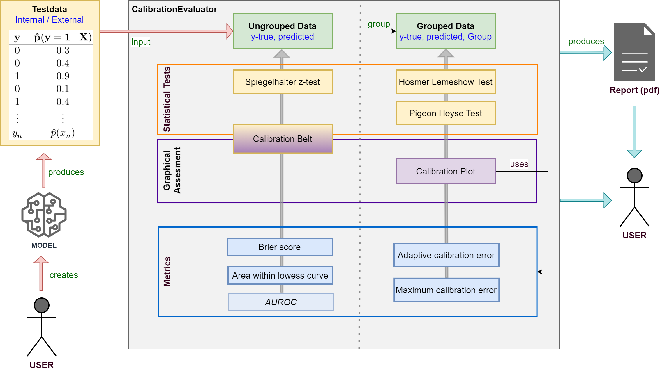
A framework for calibration evaluation of binary classification models.

When performing classification tasks you sometimes want to obtain the probability of a class label instead of the class label itself. For example, it might be interesting to determine the risk of cancer for a patient. It is desireable to have a calibrated model which delivers predicted probabilities very close to the actual class membership probabilities. For this reason, this framework was developed allowing users to measure the calibration of binary classification models.

Evaluate the calibration of binary classification models with probabilistic output (LogisticRegression, SVM, NeuronalNets …).
Apply your model to testdata and use true class labels and predicted probabilities as input for the framework.
Various statistical tests, metrics and plots are available.
Supports creating a calibration report in pdf-format for your model.

See the documentation for detailed information about classes and methods.

Installation

$ pip install pycaleva

or build on your own

$ git clone https://github.com/MartinWeigl/pycaleva.git
$ cd pycaleva
$ python setup.py install

Requirements

numpy>=1.17
scipy>=1.3
matplotlib>=3.1
tqdm>=4.40
pandas>=1.3.0
statsmodels>=0.13.1
fpdf2>=2.5.0
ipython>=7.30.1

Usage

Import and initialize

from pycaleva import CalibrationEvaluator
ce = CalibrationEvaluator(y_test, pred_prob, outsample=True, n_groups='auto')

Apply statistical tests

ce.hosmerlemeshow()     # Hosmer Lemeshow Test
ce.pigeonheyse()        # Pigeon Heyse Test
ce.z_test()             # Spiegelhalter z-Test
ce.calbelt(plot=False)  # Calibrationi Belt (Test only)

Show calibration plot
```
ce.calibration_plot()
```
Show calibration belt
```
ce.calbelt(plot=True)
```
Get various metrics
```
ce.metrics()
```

Create pdf calibration report

ce.calibration_report('report.pdf', 'my_model')

See the documentation of single methods for detailed usage examples.

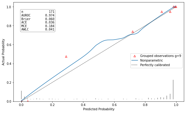
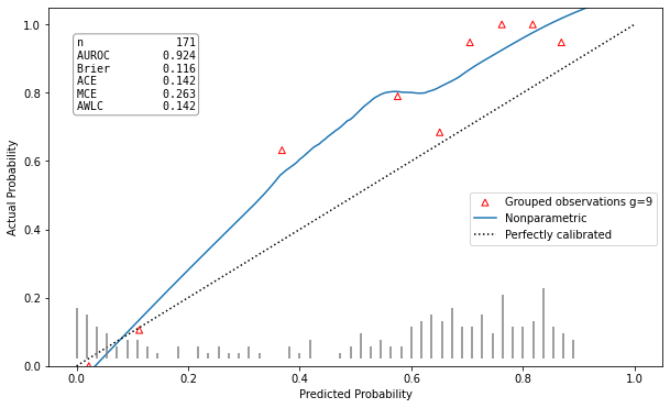
Example Results

Well calibrated model	Poorly calibrated model


hltest_result(statistic=4.982635477424991, pvalue=0.8358193332183672, dof=9)	hltest_result(statistic=26.32792475118742, pvalue=0.0018051545107069522, dof=9)
ztest_result(statistic=-0.21590257919669287, pvalue=0.829063686607032)	ztest_result(statistic=-3.196125145498827, pvalue=0.0013928668407116645)

Features

Statistical tests for binary model calibration
- Hosmer Lemeshow Test
- Pigeon Heyse Test
- Spiegelhalter z-test
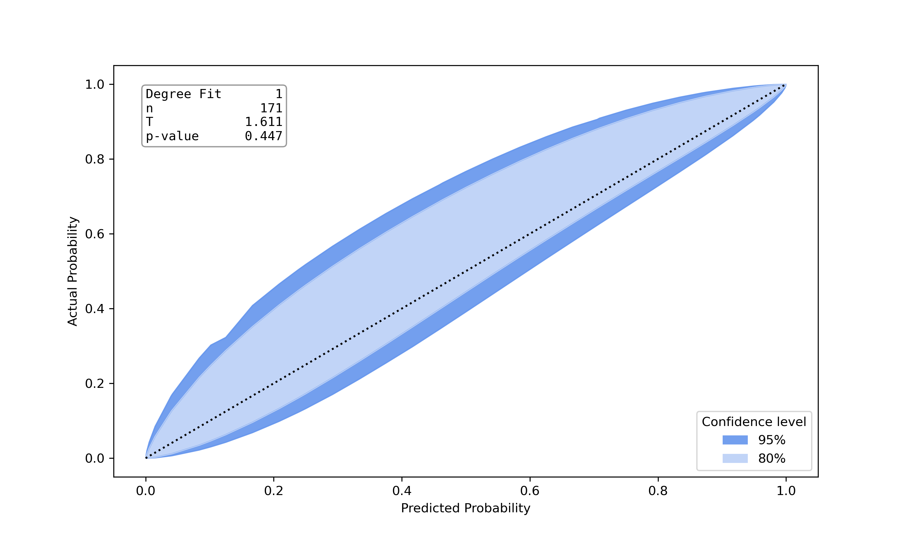
- Calibration belt
Graphical represantions showing calibration of binary models
- Calibration plot
- Calibration belt
Various Metrics
- Brier Score
- Adaptive Calibration Error
- Maximum Calibration Error
- Area within LOWESS Curve
- (AUROC)

The above features are explained in more detail in PyCalEva’s documentation

References

Statistical tests and metrics:

[1] Hosmer Jr, David W., Stanley Lemeshow, and Rodney X. Sturdivant. Applied logistic regression. Vol. 398. John Wiley & Sons, 2013.

[2] Pigeon, Joseph G., and Joseph F. Heyse. An improved goodness of fit statistic for probability prediction models. Biometrical Journal: Journal of Mathematical Methods in Biosciences 41.1 (1999): 71-82.

[3] Spiegelhalter, D. J. (1986). Probabilistic prediction in patient management and clinical trials. Statistics in medicine, 5(5), 421-433.

[4] Huang, Y., Li, W., Macheret, F., Gabriel, R. A., & Ohno-Machado, L. (2020). A tutorial on calibration measurements and calibration models for clinical prediction models. Journal of the American Medical Informatics Association, 27(4), 621-633.
Calibration plot:

[5] Jr, F. E. H. (2021). rms: Regression modeling strategies (R package version 6.2-0) [Computer software]. The Comprehensive R Archive Network. Available from https://CRAN.R-project.org/package=rms
Calibration belt:

[6] Nattino, G., Finazzi, S., & Bertolini, G. (2014). A new calibration test and a reappraisal of the calibration belt for the assessment of prediction models based on dichotomous outcomes. Statistics in medicine, 33(14), 2390-2407.

[7] Bulgarelli, L. (2021). calibrattion-belt: Assessment of calibration in binomial prediction models [Computer software]. Available from https://github.com/fabiankueppers/calibration-framework

[8] Nattino, G., Finazzi, S., Bertolini, G., Rossi, C., & Carrara, G. (2017). givitiR: The giviti calibration test and belt (R package version 1.3) [Computer software]. The Comprehensive R Archive Network. Available from https://CRAN.R-project.org/package=givitiR
Others:

[9] Sturges, H. A. (1926). The choice of a class interval. Journal of the american statistical association, 21(153), 65-66.

For most of the implemented methods in this software you can find references in the documentation as well.

Documentation API

CalibrationEvaluator

class pycaleva.calibeval.CalibrationEvaluator(y_true: numpy.ndarray, y_pred: numpy.ndarray, outsample: bool, n_groups: Union[int, str] = 10)

Bases: pycaleva._basecalib._BaseCalibrationEvaluator

Attributes

ace: Get the adaptive calibration error based on grouped data.
auroc: Get the area under the receiver operating characteristic
awlc: Get the area between the nonparametric curve estimated by lowess and the theoritcally perfect calibration given by the calibration plot bisector.
brier: Get the brier score for the current y_true and y_pred of class instance.
contingency_table: Get the contingency table for grouped observed and expected class membership probabilities.
mce: Get the maximum calibration error based on grouped data.
outsample: Get information if outsample is set.

Methods

`calbelt`([plot, subset, confLevels, alpha])	Calculate the calibration belt and draw plot if desired.
`calibration_plot`()	Generate the calibration plot for the given predicted probabilities and true class labels of current class instance.
`calibration_report`(filepath, model_name)	Create a pdf-report including statistical tests and plots regarding the calibration of a binary classification model.
`group_data`(n_groups)	Group class labels and predicted probabilities into equal sized groupes of size n.
`hosmerlemeshow`([verbose])	Perform the Hosmer-Lemeshow goodness of fit test on the data of class instance.
`merge_groups`([min_count])	Merge groups in contingency table to have count of expected and observed class events >= min_count.
`metrics`()	Get all available calibration metrics as combined result tuple.
`pigeonheyse`([verbose])	Perform the Pigeon-Heyse goodness of fit test.
`z_test`()	Perform the Spieglhalter's z-test for calibration.

property ace

Get the adaptive calibration error based on grouped data.

Returns

adaptive calibration errorfloat

property auroc

Get the area under the receiver operating characteristic

Returns

aurocfloat

property awlc

Get the area between the nonparametric curve estimated by lowess and: the theoritcally perfect calibration given by the calibration plot bisector.

Returns

Area within lowess curvefloat

property brier

Get the brier score for the current y_true and y_pred of class instance.

Returns

brier_scorefloat

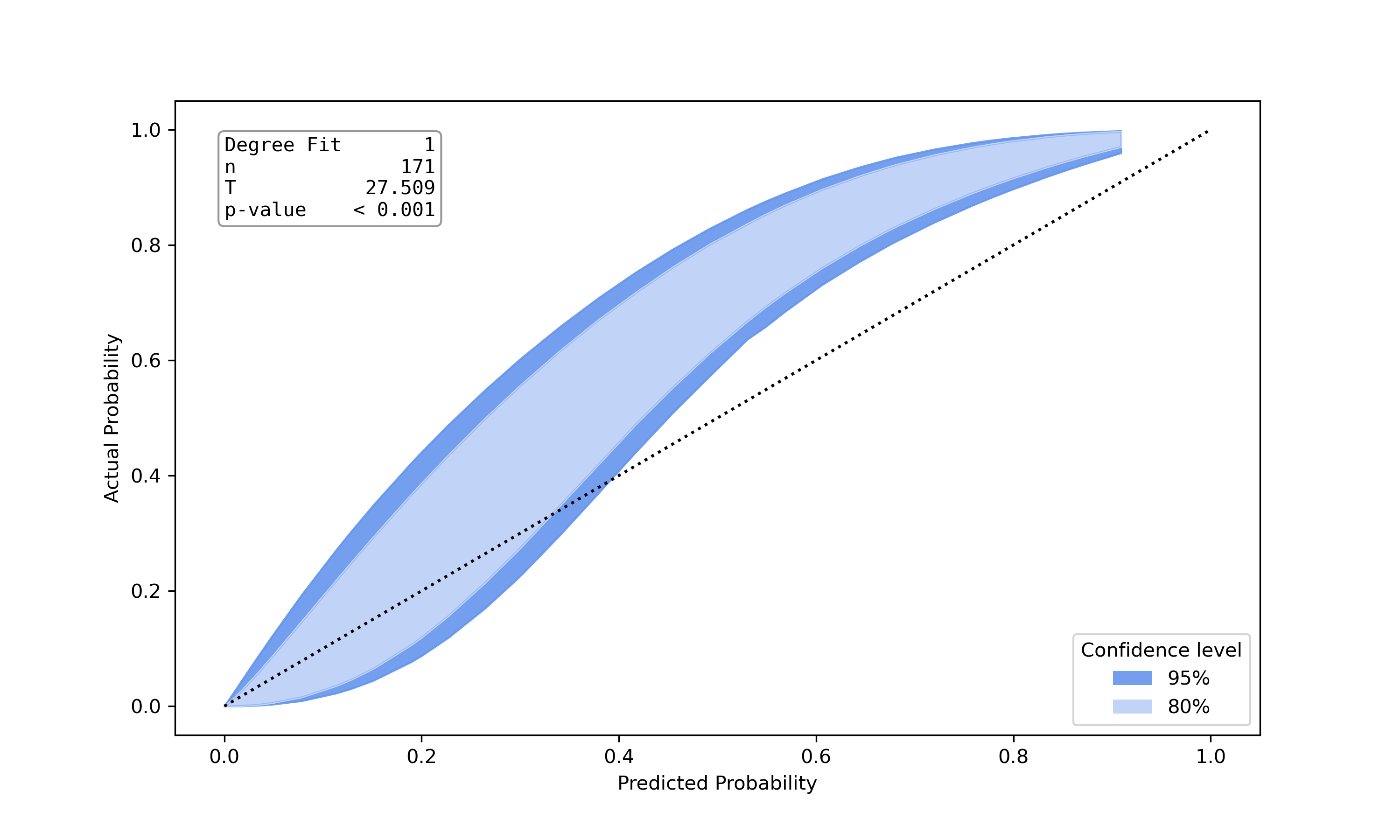
calbelt(plot: bool = False, subset=None, confLevels=[0.8, 0.95], alpha=0.95) → pycaleva._result_types.calbelt_result

Calculate the calibration belt and draw plot if desired.

Parameters

plot: boolean, optional: Decide if plot for calibration belt should be shown. Much faster calculation if set to ‘false’!
subset: array_like: An optional boolean vector specifying the subset of observations to be considered. Defaults to None.
confLevels: list: A numeric vector containing the confidence levels of the calibration belt. Defaults to [0.8,0.95].
alpha: float: The level of significance to use.

Returns

Tfloat: The Calibration plot test statistic T.
pfloat: The p-value of the test.
figmatplotlib.figure: The calibration belt plot. Only returned if plot=’True’

See also

pycaleva.calbelt.CalibrationBelt
CalibrationEvaluator.calplot

Notes

This is an implemenation of the test proposed by Nattino et al. [6]. The implementation was built upon the python port of the R-Package givitiR [8] and the python implementation calibration-belt [7]. The calibration belt estimates the true underlying calibration curve given predicted probabilities and true class labels. Instead of directly drawing the calibration curve a belt is drawn using confidence levels. A low value for the teststatistic and a high p-value (>0.05) indicate a well calibrated model. Other than Hosmer Lemeshow Test or Pigeon Heyse Test, this test is not based on grouping strategies.

References

6: Nattino, G., Finazzi, S., & Bertolini, G. (2014). A new calibration test and a reappraisal of the calibration belt for the assessment of prediction models based on dichotomous outcomes. Statistics in medicine, 33(14), 2390-2407.
7: Bulgarelli, L. (2021). calibrattion-belt: Assessment of calibration in binomial prediction models [Computer software]. Available from https://github.com/fabiankueppers/calibration-framework
8: Nattino, G., Finazzi, S., Bertolini, G., Rossi, C., & Carrara, G. (2017). givitiR: The giviti calibration test and belt (R package version 1.3) [Computer software]. The Comprehensive R Archive Network. Available from https://CRAN.R-project.org/package=givitiR

Examples

>>> from pycaleva import CalibrationEvaluator
>>> ce = CalibrationEvaluator(y_test, pred_prob, outsample=True, n_groups='auto')
>>> ce.calbelt(plot=False)
calbelt_result(statistic=1.6111330037643796, pvalue=0.4468347221346196, fig=None)

calibration_plot()

Generate the calibration plot for the given predicted probabilities and true class labels of current class instance.

Returns

plotmatplotlib.figure

See also

CalibrationEvaluator.calbelt

Notes

This calibration plot is showing the predicted class probability against the actual probability according to the true class labels as a red triangle for each of the groups. An additional calibration curve is draw, estimated using the LOWESS algorithm. A model is well calibrated, if the red triangles and the calibration curve are both close to the plots bisector. In the left corner of the plot all available metrics are listed as well. This implementation was made following the example of the R package rms [5].

References

5: Jr, F. E. H. (2021). rms: Regression modeling strategies (R package version 6.2-0) [Computer software]. The Comprehensive R Archive Network. Available from https://CRAN.R-project.org/package=rms

Examples

>>> from pycaleva import CalibrationEvaluator
>>> ce = CalibrationEvaluator(y_test, pred_prob, outsample=True, n_groups='auto')
>>> ce.calibration_plot()

calibration_report(filepath: str, model_name: str) → None

Create a pdf-report including statistical tests and plots regarding the calibration of a binary classification model.

Parameters

filepath: str: The filepath for the output file. Must end with ‘.pdf’
model_name: str: The name for the evaluated model.

property contingency_table

Get the contingency table for grouped observed and expected class membership probabilities.

Returns

contingency_tableDataFrame

group_data(n_groups: Union[int, str]) → None

Group class labels and predicted probabilities into equal sized groupes of size n.

Parameters

n_groups: int or str: Number of groups to use for grouping probabilities. Set to ‘auto’ to use sturges function for estimation of optimal group size [9].

Raises

ValueError: If the given number of groups is invalid.

Notes

Sturges function for estimation of optimal group size:

k = ⌈ \log_{2} n ⌉ + 1

Hosmer and Lemeshow recommend setting number of groups to 10 and with equally sized groups [1].

References

1: Hosmer Jr, David W., Stanley Lemeshow, and Rodney X. Sturdivant. Applied logistic regression. Vol. 398. John Wiley & Sons, 2013.
9: Sturges, H. A. (1926). The choice of a class interval. Journal of the american statistical association, 21(153), 65-66.

hosmerlemeshow(verbose=True) → pycaleva._result_types.hltest_result

Perform the Hosmer-Lemeshow goodness of fit test on the data of class instance. The Hosmer-Lemeshow test checks the null hypothesis that the number of given observed events match the number of expected events using given probabilistic class predictions and dividing those into deciles of risks.

Parameters

verbosebool (optional, default=True): Whether or not to show test results and contingency table the teststatistic relies on.

Returns

Cfloat: The Hosmer-Lemeshow test statistic.
p-valuefloat: The p-value of the test.
dofint: Degrees of freedom

See also

CalibrationEvaluator.pigeonheyse
CalibrationEvaluator.z_test
scipy.stats.chisquare

Notes

A low value for C and high p-value (>0.05) indicate a well calibrated model. The power of this test is highly dependent on the sample size. Also the teststatistic lacks fit to chi-squared distribution in some situations [3]. In order to decide on model fit it is recommended to check it’s discrematory power as well using metrics like AUROC, precision, recall. Furthermore a calibration plot (or reliability plot) can help to identify regions of the model underestimate or overestimate the true class membership probabilities.

Hosmer and Lemeshow estimated the degrees of freedom for the teststatistic performing extensive simulations. According to their results the degrees of freedom are k-2 where k is the number of subroups the data is divided into. In the case of external evaluation the degrees of freedom is the same as k [1].

Teststatistc:

$E_{k 1} = \sum_{i = 1}^{n_{k}} {\hat{p}}_{i 1}$

$O_{k 1} = \sum_{i = 1}^{n_{k}} y_{i 1}$

$\hat{C} = \sum_{k = 1}^{G} \frac{{(O_{k 1} - E_{k 1})}^{2}}{E_{k 1}} + \frac{{(O_{k 0} - E_{k 0})}^{2}}{E_{k 0}}$

References

1: Hosmer Jr, David W., Stanley Lemeshow, and Rodney X. Sturdivant. Applied logistic regression. Vol. 398. John Wiley & Sons, 2013.
10: “Hosmer-Lemeshow test”, https://en.wikipedia.org/wiki/Hosmer-Lemeshow_test
11: Pigeon, Joseph G., and Joseph F. Heyse. “A cautionary note about assessing the fit of logistic regression models.” (1999): 847-853.

Examples

>>> from pycaleva import CalibrationEvaluator
>>> ce = CalibrationEvaluator(y_test, pred_prob, outsample=True, n_groups='auto')
>>> ce.hosmerlemeshow()
hltest_result(statistic=4.982635477424991, pvalue=0.8358193332183672, dof=9)

property mce

Get the maximum calibration error based on grouped data.

Returns

maximum calibration errorfloat

merge_groups(min_count: int = 1) → None

Merge groups in contingency table to have count of expected and observed class events >= min_count.

Parameters

min_countint (optional, default=1)

Notes

Hosmer and Lemeshow mention the possibility to merge groups at low samplesize to have higher expected and observed class event counts [1]. This should guarantee that the requirements for chi-square goodness-of-fit tests are fullfilled. Be aware that the power of tests will be lower after merge!

References

1: Hosmer Jr, David W., Stanley Lemeshow, and Rodney X. Sturdivant. Applied logistic regression. Vol. 398. John Wiley & Sons, 2013.

metrics()

Get all available calibration metrics as combined result tuple.

Returns

aurocfloat: Area under the receiver operating characteristic.
brierfloat: The scaled brier score.
aceint: Adaptive calibration error.
mcefloat: Maximum calibration error.
awlcfloat: Area within the lowess curve

Examples

>>> from pycaleva import CalibrationEvaluator
>>> ce = CalibrationEvaluator(y_test, pred_prob, outsample=True, n_groups='auto')
>>> ce.metrics()
metrics_result(auroc=0.9739811912225705, brier=0.2677083794415594, ace=0.0361775962446639, mce=0.1837227304691177, awlc=0.041443052220213474)

property outsample

Get information if outsample is set. External validation if set to ‘True’.

Returns

Outsample statusbool

pigeonheyse(verbose=True) → pycaleva._result_types.phtest_result

Perform the Pigeon-Heyse goodness of fit test. The Pigeon-Heyse test checks the null hypothesis that number of given observed events match the number of expected events over divided subgroups. Unlike the Hosmer-Lemeshow test this test allows the use of different grouping strategies and is more robust against variance within subgroups.

Parameters

verbosebool (optional, default=True): Whether or not to show test results and contingency table the teststatistic relies on.

Returns

Jfloat: The Pigeon-Heyse test statistic J².
pfloat: The p-value of the test.
dofint: Degrees of freedom

See also

CalibrationEvaluator.hosmerlemeshow
CalibrationEvaluator.z_test
scipy.stats.chisquare

Notes

This is an implemenation of the test proposed by Pigeon and Heyse [2]. A low value for J² and high p-value (>0.05) indicate a well calibrated model. Other then the Hosmer-Lemeshow test an adjustment factor is added to the calculation of the teststatistic, making the use of different grouping strategies possible as well.

The power of this test is highly dependent on the sample size. In order to decide on model fit it is recommended to check it’s discrematory power as well using metrics like AUROC, precision, recall. Furthermore a calibration plot (or reliability plot) can help to identify regions of the model underestimate or overestimate the true class membership probabilities.

Teststatistc:

$ϕ_{k} = \frac{\sum_{i = 1}^{n_{k}} {\hat{p}}_{i 1} (1 - {\hat{p}}_{i 1})}{n_{k} {\bar{p}}_{k 1} (1 - {\bar{p}}_{k 1})}$

$J^{2} = \sum_{k = 1}^{G} \frac{{(O_{k 1} - E_{k 1})}^{2}}{ϕ_{k} E_{k 1}} + \frac{{(O_{k 0} - E_{k 0})}^{2}}{ϕ_{k} E_{k 0}}$

References

1: Hosmer Jr, David W., Stanley Lemeshow, and Rodney X. Sturdivant. Applied logistic regression. Vol. 398. John Wiley & Sons, 2013.
2: Pigeon, Joseph G., and Joseph F. Heyse. “An improved goodness of fit statistic for probability prediction models.” Biometrical Journal: Journal of Mathematical Methods in Biosciences 41.1 (1999): 71-82.
11: Pigeon, Joseph G., and Joseph F. Heyse. “A cautionary note about assessing the fit of logistic regression models.” (1999): 847-853.

Examples

>>> from pycaleva import CalibrationEvaluator
>>> ce = CalibrationEvaluator(y_test, pred_prob, outsample=True, n_groups='auto')
>>> ce.pigeonheyse()
phtest_result(statistic=5.269600396341568, pvalue=0.8102017228852412, dof=9)

z_test() → pycaleva._result_types.ztest_result

Perform the Spieglhalter’s z-test for calibration.

Returns

statisticfloat: The Spiegelhalter z-test statistic.
pfloat: The p-value of the test.

See also

CalibrationEvaluator.hosmerlemeshow
CalibrationEvaluator.pigeonheyse

Notes

This calibration test is performed in the manner of a z-test. The nullypothesis is that the estimated probabilities are equal to the true class probabilities. The test statistic under the nullypothesis can be approximated by a normal distribution. A low value for Z and high p-value (>0.05) indicate a well calibrated model. Other than Hosmer Lemeshow Test or Pigeon Heyse Test, this test is not based on grouping strategies.

Teststatistc:

$Z = \frac{\sum_{i = 1}^{n} (y_{i} - {\hat{p}}_{i}) (1 - 2 {\hat{p}}_{i})}{\sqrt{\sum_{i = 1}^{n} {(1 - 2 {\hat{p}}_{i})}^{2} {\hat{p}}_{i} (1 - {\hat{p}}_{i})}}$

References

1: Spiegelhalter, D. J. (1986). Probabilistic prediction in patient management and clinical trials. Statistics in medicine, 5(5), 421-433.
2: Huang, Y., Li, W., Macheret, F., Gabriel, R. A., & Ohno-Machado, L. (2020). A tutorial on calibration measurements and calibration models for clinical prediction models. Journal of the American Medical Informatics Association, 27(4), 621-633.

Examples

>>> from pycaleva import CalibrationEvaluator
>>> ce = CalibrationEvaluator(y_test, pred_prob, outsample=True, n_groups='auto')
>>> ce.z_test()
ztest_result(statistic=-0.21590257919669287, pvalue=0.829063686607032)

CalibrationBelt

class pycaleva.calbelt.CalibrationBelt(y_true: numpy.ndarray, y_pred: numpy.ndarray, outsample: bool, subset=None, confLevels=[0.8, 0.95], alpha=0.95)

Bases: object

Methods

`plot`([alpha])	Draw the calibration belt plot.
`stats`()	Get the calibration belt test result, withour drawing the plot.

plot(alpha=0.95, **kwargs)

Draw the calibration belt plot.

Parameters

alpha: float, optional: Sets the significance level.
confLevels: list, optional: Set the confidence intervalls for the calibration belt. Defaults to [0.8,0.95].

Returns

Tfloat: The Calibration plot test statistic T.
pfloat: The p-value of the test.
figmatplotlib.figure: The calibration belt plot. Only returned if plot=’True’

See also

CalibrationEvaluator.calbelt

Notes

This is an implemenation of the test proposed by Nattino et al. [6]. The implementation was built upon the python port of the R-Package givitiR [8] and the python implementation calibration-belt [7]. The calibration belt estimates the true underlying calibration curve given predicted probabilities and true class labels. Instead of directly drawing the calibration curve a belt is drawn using confidence levels. A low value for the teststatistic and a high p-value (>0.05) indicate a well calibrated model. Other than Hosmer Lemeshow Test or Pigeon Heyse Test, this test is not based on grouping strategies.

References

6: Nattino, G., Finazzi, S., & Bertolini, G. (2014). A new calibration test and a reappraisal of the calibration belt for the assessment of prediction models based on dichotomous outcomes. Statistics in medicine, 33(14), 2390-2407.
7: Bulgarelli, L. (2021). calibrattion-belt: Assessment of calibration in binomial prediction models [Computer software]. Available from https://github.com/lbulgarelli/calibration
8: Nattino, G., Finazzi, S., Bertolini, G., Rossi, C., & Carrara, G. (2017). givitiR: The giviti calibration test and belt (R package version 1.3) [Computer software]. The Comprehensive R Archive Network. Available from https://CRAN.R-project.org/package=givitiR

Examples

>>> from pycaleva.calbelt import CalibrationBelt
>>> cb = CalibrationBelt(y_test, pred_prob, outsample=True)
>>> cb.plot()
calbelt_result(statistic=1.6111330037643796, pvalue=0.4468347221346196, fig=matplotlib.figure)

stats()

Get the calibration belt test result, withour drawing the plot.

Returns

Tfloat: The Calibration plot test statistic T.
pfloat: The p-value of the test.

Notes

A low value for the teststatistic and a high p-value (>0.05) indicate a well calibrated model.

Examples

>>> from pycaleva.calbelt import CalibrationBelt
>>> cb = CalibrationBelt(y_test, pred_prob, outsample=True)
>>> cb.stats()
calbelt_result(statistic=1.6111330037643796, pvalue=0.4468347221346196, fig=None)

Example Usage

See this notebook for example usage.

Development

This framework is still under development and will be improved over time. Feel free to report any issues at the project homepage.